16. Fair value estimation#
16.1. Introduction#
In this chapter we introduce techniques to estimate the fair value of a financial instrument exploiting the pricing information available in financial markets. The fair value is a theoretical concept that tries to remove from prices observed in the market all the idiosyncratic components like transaction costs, dealer spreads and skews, liquidity premiums, etc. The remaining price or fair value would be the price at which market participants would theoretically trade in perfect markets, where there are not trading frictions. When instruments trade in liquid markets, we can use statistical techniques like Kalman filters to remove these components, which are modeled as noise on top of the theoretical fair value. When the instruments are not frequently, those estimations might have large uncertainties, and economical models, if available, are used in combination with the available pricing information to estimate the fair value. A particular relevant case are models for derivatives pricing based on non-arbitrage conditions. These models, based on the award-winning Black-Scholes-Merton theory, exploit information from the underlyings in the derivatives in combination with non-arbitrage constraints to estimate the fair value.
16.2. Pricing of flow products#
For flow products that are relatively liquid, we can aim at extracting all the pricing information from price indications and trades in the market, without having to resort to economic theories of fair value. In this setup, we consider their price the one that market participants are willing to pay for.
The issue, though, is that price indications and trades cannot be considered themselves pure observations of fair value, since they might be affected by market frictions: bid ask spreads, particularities of the negotiation mechanism, liquidity fluctuations, specific needs of market participants at a given time, etc. When instruments trade in limit order books, a popular estimation of the fair value is using the mid-price, the arithmetic average of the best bid and ask. However, if bid-ask spreads are wide of liquidity is thin in the first levels, such estimation is not necessary very precise. Trades provide a lot of information, since they are real transaction and not indications of interests, the larger they are in principle the more information. Still, they are subject to the aforementioned market frictions that reduce their reliability.
These makes all these price observations noisy estimates of the fair value, so if we want to estimate a fair value out of them we need to be able to separate the signal from the noise, or in other words, filter those observations. This is precisely what, under certain model assumptions, a Kalman filter does.
16.2.1. The Kalman Filter model for pricing#
The Kalman filter was introduced in the chapter on Bayesian Theory. It is a Bayesian filtering algorithm that allows to perform exact inference, i.e. compute the closed-form distribution, of the latent state vector in a Linear Gaussian State Space Model (LG-SSM).
Recall that a State Space Model (SSM) is a model to describe dynamic systems where we have a non or partially observable state, a vector \(\mathbf{x}\), whose dynamics in time is described by a so-called transition equation:
where \(f(\mathbf{x}_t, \mathbf{u}_t)\) is a general function, \(\mathbf{u}_t\) are inputs (or controls) that affect the dynamics, \(\Delta t\) is the time-step between observations, and \(\mathbf{ \epsilon}_t\) is a transition noise with a given distribution. The state is observed indirectly via a proxy vector \(\mathbf{y}\) via the observation equation:
where \(g(\mathbf{x}_t, \mathbf{u}_t)\) is another general function and \(\mathbf{\eta}_t\) the observation noise, meaning that observations have a degree of uncertainty with respect to the latent space.
A Linear Gaussian Model (LGM) is a specific case of the SSM were both the transition and observation functions are linear and the noise terms are Gaussian. In this case, we can use the Kalman filter algorithm to compute the distribution of the state vector at any time, given the observations and the transition and observation model. If some or all the parameters of these models are not known, they can be estimated using standard techniques like Maximum Likelihood Estimation (MLE) or Expectation Maximization (EM) when the former becomes computationally intractable due to the latent state vector.
For non-Linear Gaussian Models, there are extensions of the Kalman filter that can be used:
Extended Kalman Filter (EKF): Extends the Kalman Filter to non-linear state space models by linearizing the dynamics and observation models around the current estimate using Taylor expansions.
Unscented Kalman Filter (UKF): Avoids linearization by using deterministic sampling to approximate the state distribution.
16.2.1.1. A simple pricing model#
Let us consider a simple setup where we aim to infer the distribution of the mid-price \(m_t\) of a financial instrument that follows a random walk:
We don’t observe this mid-price, only trades which we consider noisy observation of the mid since they include transaction costs and potentially other external factors like dealer inventory positions, etc:
Readers will recognize that this is the local level model discussed extensively in the Chapter on Bayesian Modelling. For the observation noise we can introduce prior business knowledge about the confidence we have on trade observations as a source of pricing information. In his Option Trading’s book, Euan Sinclair describes a simple model that quantifies the information provided by trades based on the size of the trade, \(v\):
where \(\sigma_p\) is a baseline observation noise and \(v_\text{max}\) is an input to the model, the trade size we believe saturates information the information provided in the sense that our mid estimation will essentially move the price of the trade. In contrast, trades of small size, \(v \ll v_\text{max}\), will have \(\sigma_p \rightarrow \infty\) and will provide a negligible pricing information. An alternative simple model is:
where \(v_0\) in this case is a size scale that separates the regimes where the information provided by the trade is negligible, \(v \ll v_0\), or relevant \(v \gg v_0\), but it does not saturate for a specific trading size, as in Sinclair’s model. Of course nothing prevents to use more business prior knowledge to enrich the observation model with other observable characteristics of the trade or the wider market context.
16.2.1.2. Estimation of the simple pricing model#
As discussed in Bayesian Modelling, the standard way to estimate the parameters of a Kalman Filter is using the Expectation Maximization (EM) algorithm, suitable for probabilistic models with latent variables. However, the properties of the simple pricing model can be exploited to obtain closed-form estimators for its parameters using moment matching.
Let us start by working with a model where observation errors have no dependency on the volume: \(\sigma_\nu (v) = \sigma_\nu\). The key is to compute statistics of:
which depend only on observed trades. First we compute the variance:
where we have used that \(\epsilon_t\), \(\nu_{t+\Delta t}\) and \(\nu_t\) are independent random variables. This expression links the variance of the first differences in trade prices with the parameters to estimate. We need though a second expression to solve for each parameters separately. For that we compute the lag-1 auto-covariance of \(d_t\):
where again we have used the independence between the noise terms. Our estimators read then:
The results have an interesting interpretation:
Starting from the first equation: the variance of the mid-price must be lower than the variance of the observed trades, given the additional noise in the observation equation. Or, in other words, since the mid-price is filtered from the trades, which means that we estimate it by removing noise from the trades, it has to have a lower variance.
The second equation can be recognized as a form of the Roll estimator for effective bid-ask spreads, a typical measure of liquidity. Of course, by construction of the model, the noise that is filtered is essentially the bid-ask spread that liquidity providers request as a compensation for the liquidity provision.
In the case of volume dependent observation errors, we can still compute these statistics, which now read:
The statistical estimator of the variance of the first differences can still be used, by accounting by the variability of the error with volume (heteroskedasticity):
Moving into the 1-lag covariance, we have:
As far as we the volume dependency has a single parameter to fit, we can still use these two equations to solve for the parameters. If we use, for instance, the simple model \(\sigma_\nu(v) = \sigma_p \frac{v_0}{v}\), where \(v_0\) is given and \(\sigma_p\) is to be estimated from data (notice that we could simply estimate \(\sigma_p v_0\), the factorization is useful for business interpretation):
In this simple case, the estimation of the parameters \(\sigma_p\) and \(\sigma_\epsilon\) is straightforward. More complex functions like the one from Sinclair cannot be estimated with only two moments. Further moments can be computed to provide extra equations, although at this point it might be worthy to resort to standard estimation techniques like EM if available.
16.2.1.3. Inference on the simple pricing model#
We can use the general Kalman filter equations described in Bayesian Modelling to derive the distribution of our mid - price at the next time \(t + \Delta t\) where a trade happens.
The Kalman filter algorithm operates sequentially over observation steps applying two steps, the predict step, where we compute the distribution of the mid-price based purely on the random walk model, and the update step in which we incorporate the information provided by the observation of a new trade. We define \(m_{t+\Delta t}^t\) as the distribution of the mid-price at \(t+\Delta t\) before observing the trade, and \(m_{t+\Delta}^{t+\Delta t}\) afterwards.
Let us apply first the predict step. The distribution of \(m_{t+\Delta t}^t\) is Gaussian with mean and variance given by:
Since our model uses a drift-less random walk dynamics for the evolution of the mid-price, the updated mean does not change and the variance increases proportionally to the time step \(\Delta t\).
Now we use the update step to incorporate the information from a trade happening at \(t + \Delta t\):
where \(K_t\) is the Kalman gain, given by:
The updated mean is an interpolation between the predicted mean and the trade observation, weighted by the Kalman gain
If the observation noise is much smaller than the uncertainty in the mean in the prediction step, namely \(\sigma_\eta \ll \sigma_{m,t+\Delta t}^t\), the Kalman gain then tends to \(K_t \rightarrow 1\) and \(\bar{m}_{t+\Delta t}^{t+\Delta t} = p_{t+\Delta t}\), i.e. since our confidence on the information from the trade is much higher than our best estimation of the mean, we essentially update the mean with the trade price.
On the contrary, if \(\sigma_\eta \gg \sigma_{m,t+\Delta t}^t\), the Kalman gain then tends to \(K_t \rightarrow 0\) and \(\bar{m}_{t+\Delta t}^{t+\Delta t} = \bar{m}_{t}^{t+\Delta t}\). In this case, our confidence on the information provided by the trade is very low, so essentially we ignore the trade information and use the predicted mean.
In between those two limiting cases, the updated mean combines the information from the prediction using the internal dynamics and our last update, and the trade information.
If we look at the new standard deviation, we also find similar limiting behaviors:
If \(\sigma_\eta \ll \sigma_{m,t+\Delta t}\), then \(\sigma_{m,t+\Delta t}^{t+\Delta t} \rightarrow \sigma_\eta\), since as we discussed above, we essentially use the trade information to inform our estimation of the mid.
If \(\sigma_\eta \gg \sigma_{m,t+\Delta t}\), then \(\sigma_{m,t+\Delta t}^{t+\Delta t} \rightarrow \sigma_{m,t+\Delta t}^t\), i.e. we stick with the estimation from the predict step
One interesting consequence of the optimality of the Kalman filter is that the updated standard deviation cannot be larger than the predicted one, and for any finite \(\sigma_\eta\) is always smaller: the information from the trade always contributes to improve our estimation of the mid-price. This is easily seen writing:
Since \(\frac{\sigma_{m,t+\Delta t}^t}{\sigma_\eta}\) is non-negative, then the denominator is never lower than 1.
In some applications of the local level model to pricing we might also be interested in the Kalman smoothing algorithm. Recall that the difference with the Kalman filtering we have just seen is that in smoothing we estimate the latent variable using all the available data, including the future. Of course this means Kalman smoothing does not make sense for online price inference, but there are other applications of this pricing model where using the best estimation of the latent mid-price is relevant:
Estimation of parameters when using Expectation Maximization, as discussed in in Bayesian Modelling
Calibration of pricing models, for instance as we will discuss in the chapter on RfQ Modelling, when we seek to estimate the hit rate probability, or the probability that a client trades an RfQ from a dealer given the quoted price. In this case, we are interested in having the best estimation possible of the mid-price to isolate the effect of the spread, which is the one that puts dealers in competition. In the same chapter we will also discuss models to evaluate the toxicity of clients’ flows, i.e. when clients seem to have more information than the dealer when trading, so the dealer seems to be later in the wrong side of the market. Estimating such models typically relies on analyzing how the mid-price of the instrument moves before and after a client intends to trade.
16.2.1.4. Multiple observations of the same instrument#
In many real pricing situations, we might have different sources that reveal information about the fair value of an instrument, for example trades in different platforms, information from composites, or pricing information derived indirectly from trading indicators like the hit&miss. We will explore later those sources in detail. If they happen asynchronously, we can just use the simple pricing model introduced in the previous section, adjusting the observation error depending on the pricing source.
If they happen synchronously, though, we need to expand the Kalman filter to cope with simultaneous observations. This requires to change the observation model to a system of equations:
We can compute the Kalman gain in this case, which is a vector matrix:
where:
is the total observation precision. Notice that, as a sanity check, in the case of a single observation we recover the Kalman gain derived in the previous section. For multiple observations, the update equation then reads:
The relative weight of influence of each observation depends on the fraction of the total variance that the observation variance represents, with more noisy observations having a smaller effect in the update.
16.2.1.5. Multiple correlated instruments#
The Kalman filter model for pricing becomes even more relevant when we include information from other financial instruments that are historically correlated with the one whose mid-price we are estimated. Typical situations are:
Instruments that are more liquid, i.e. they trade more often and with smaller bid and ask spreads. This allows us to improve the estimation of the mid-price until we observe a new trade from the instrument, anticipating potential relevant movements derived from common market factors.
Instruments that trade in markets that are open when markets where our instrument of interest is traded are closed. This allows us to reduce the uncertainty from the overnight gap in trading data.
The simple pricing model we have analyzed so far can be easily extended to include information from a set of N instruments. Notice that in this case what we are actually doing is estimating the mid-prices of all the instruments in the set, not necessarily only the one of interest. The evolution of the mid-prices is now modelled using:
where \(\Sigma_\epsilon\) is now a covariance matrix that takes into account the effect of correlations in the pricing movements. Price observations follow the model:
In this case, since we are already modelling correlations at mid-price level, a typical choice is to take \(\Sigma_\nu\) diagonal, i.e. \(\Sigma_\nu = \text{diag}(\sigma_{\nu,1}^2, ..., \sigma_{\nu_N}^2)\), although in certain setups one might want to include some of form of bid-ask spread correlation between instruments.
With this model specification, we can directly use the filtering, smoothing and EM equations discussed in the Bayesian Modelling chapter. Let us though specifically focus on the case of \(N=2\) instruments, where we can work out in detail the Kalman filter equations to get further insights into the model’s inner workings.
The predict step in the Kalman filter is given by the following equations:
which are relatively simple, as expected. The update step equations are more interesting, since they include the effect of observations, and critically the impact of one instrument’s trades into the mid-price or the other:
with the Kalman gain being:
For the two instrument case, the Kalman gain can be expanded into:
Let us analyze some particular cases:
If we set the correlation to zero, \(\rho_t^{t-1} = 0\), the Kalman gain becomes:
\[\begin{split}\begin{aligned} K_t = \frac{1}{(\sigma_{\nu,1}^2 + (\sigma_{1,t}^{t-1})^2)(\sigma_{\nu,2}^2 + (\sigma_{2,t}^{t-1})^2)} \nonumber \\ \begin{pmatrix} (\sigma_{1,t}^{t-1})^2 \sigma_{\nu,2}^2 + (\sigma_{1,t}^{t-1})^2(\sigma_{2,t}^{t-1})^2 & 0 \\ 0 & (\sigma_{2,t}^{t-1})^2\sigma_{\nu,1}^2 + (\sigma_{1,t}^{t-1})^2 (\sigma_{2,t}^{t-1})^2 \end{pmatrix} \\ \nonumber = \begin{pmatrix} \frac{(\sigma_{1,t}^{t-1})^2}{\sigma_{\nu,1}^2 + (\sigma_{1,t}^{t-1})^2} & 0 \\ 0 & \frac{(\sigma_{2,t}^{t-1})^2}{\sigma_{\nu,2}^2 + (\sigma_{2,t}^{t-1})^2} \end{pmatrix} \nonumber \end{aligned}\end{split}\]i.e. we recover the equations of the Kalman gain for a single instrument for each diagonal, and the update equation factors in two independent updates.
If we set \(\sigma_{\nu, 1}^{-1} = 0\), which simulates the case in which we don’t have an observation of a trade in the first financial instrument –by considering its observation error so large that it’s effect is negligible, the Kalman gain becomes:
\[\begin{split}\begin{aligned} K_t = \begin{pmatrix} 0 & \frac{\rho_t^{t-1} \sigma_{1,t}^{t-1}\sigma_{2,t}^{t-1}}{\sigma_{\nu,2}^2 + (\sigma_{2,t}^{t-1})^2} \\ 0 & \frac{(\sigma_{2,t}^{t-1})^2}{\sigma_{\nu,2}^2 + (\sigma_{2,t}^{t-1})^2} \nonumber \\ \end{pmatrix} \end{aligned}\end{split}\]The update equations for each instruments mid-price read:
\[m_{1,t|t} = m_{1,t|t-1} + \frac{\rho_t^{t-1} \sigma_{1,t}^{t-1}\sigma_{2,t}^{t-1}}{\sigma_{\nu,2}^2 + (\sigma_{2,t}^{t-1})^2} (m_{2,t|t-1} - P_{2,t + \Delta t})\]\[m_{2,t|t} = m_{2,t|t-1} + \frac{(\sigma_{2,t}^{t-1})^2}{\sigma_{\nu,2}^2 + (\sigma_{2,t}^{t-1})^2} (m_{2,t|t-1} - P_{2,t + \Delta t}) \]Notice that these equations are equivalent to the ones that we would derive if we use an observation matrix \(H = (0, 1)\) and compute the update step for arbitrary values of the parameters. Going into the results, the second equation is the same update equation we had for a single instrument for which we have observed a trade. The first equation is more interesting, since it isolates the effect that an observation of a trade in an instrument has in our mid-price estimation of a correlated instrument. As expected, the influence is proportional to the estimated correlation between the instruments, \(\rho_t^{t-1}\). The effect of the influence depends on the relative sizes of the variances in play. It helps to rewrite the equation as:
\[m_{1,t|t} = m_{1,t|t-1} + \beta_{12,t}^{t-1} \frac{1}{1+ \frac{\sigma_{\nu,2}^2}{ (\sigma_{2,t}^{t-1})^2}} (m_{2,t|t-1} - P_{2,t + \Delta t})\]where \(\beta_{12,t}^{t-1} \equiv \frac{\rho_t^{t-1} \sigma_{1,t}^{t-1}}{\sigma_{2,t}^{t-1}}\) is the linear regression coefficient between \(m_{1,t}\) and \(m_{2,t}\). It provides an upper bound on the Kalman gain between the two instruments, which happens when the observation in the second instrument has no error \(\sigma_{\nu, 2} = 0\). This makes sense, since in the absence of noise in the observation of the second instrument, the update equation becomes the best linear prediction of \(m_{1,t}\) using \(m_{2,t}\).
Let’s evaluate this model in one of the typical scenarios for fair value discovery discussed above: two correlated instruments traded in markets with some periods of non-overlapping trading. The objective is to leverage their correlation to estimate fair values for the instrument whose market is closed. The underlying principle is that new information affecting the price of the actively traded instrument during its market hours would similarly impact the closed-market instrument, if it were tradable.
For that, we first generate synthetic mid-prices using a correlated Brownian motion with \(\rho = 0.9\), \(\sigma_1 = 5e-4\) and \(\sigma_2 = 4e-4\). Then we generate trades over 22 days but for each day, each day consisting on 60 time-steps to make the simulation efficient. We consider three situations: one in which only the first instrument is traded, on in which only the second instrument is traded, and a third one in which both are simultaneously traded. We use a diagonal observation covariance to generate the trades, i.e. we assume that there is no correlation between the spreads with respect to the mid, so correlation is driven exclusively by mid-price correlations. To generate the trades, we use standard deviations in the observation covariance of \(0.032\) and \(0.045\), respectively. Then we use Expectation Maximization (EM) over the first half of the synthetic trade data to estimate the parameters of the model, and run the Kalman filter over the second half of the data to compare the estimations of the mid-price to the real simulated values. The results can be seen in the following figure:
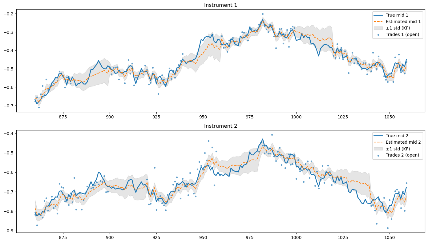
Fig. 16.1 Estimation of the fair value of instruments when their market is closed, using information from correlated instrument that trade at those times. The results are based on a simulation in which first the mid-prices are generated (blue lines) and trades (blue dots) are simulated when the market is open, which. happens half of the day. Notice that a third of the day both instruments trade simultaneously. The orange line are the mid-prices estimated using the Kalman filter, which is trained with half of the data using EM and the run over the second half of the data. The figure focus on four days of test data.#
As we see, the Kalman filter successfully exploits the correlation between instruments to update the mid-price of the instruments when the market is closed. The updates are not perfect but they capture the overnight trends, improving over typical baselines like the closing price of the instrument. In general, the estimated mid-prices include the true mid-prices within one standard deviation, depicted as the shaded grey area in the figure.
16.2.2. Pricing sources and models#
When it comes to feeding the Kalman filter with information to improve the estimations of the fair value, there is a variety of sources that is typically used. Let us discuss the most typical sources, those based on Limit Order Book (LOB) data and those based on Request for Quote (RfQ) data. As we have seen, these sources can be used both if they belong to the instrument of interest or correlated ones. However, there are some considerations to take into account when using correlated instruments, which we discuss in the end.
One point that will become a common theme in this section is the information content of the observations. Intuitively, not every source of pricing is equally informative. For example, as we discussed above, we expect that trades with larger volumes are more informative than small trades. In the same way, a cancellation of a limit order deep in a Limit Order Book might not carry meaningful new pricing information. These effects need to be incorporated case by case into the pricing model.
16.2.2.1. LOB traded#
Limit Order Books (LOBs) are complex structures that contain extensive pricing information. Nevertheless, as discussed in Chapter market_microstructure, the primary references for price discovery are the best bid and ask quotes, the mid-price—defined as the average of these two—and the prices of executed trades. To improve robustness and reduce the impact of potential market manipulation, it is standard practice to compute volume-weighted averages of the first K levels on both the bid and ask sides, and to define a robust mid-price based on these averages.
16.2.2.1.1. Mid-price information#
As mentioned above, a robust mid-price indicator in a LOB is:
where \(v_{b/a, i}\) and \(P_{b/a, i}\) are volumes and prices of bid and ask, respectively, and \(K\) is the number of levels that are taken into account, for instance \(K = 4\). We have omitted the time subscript in volumes and prices but they are also time dependent. Similarly, we can compute a robust bid-ask spread in the form:
which has to be positive since any bid and ask limit orders with the same price are automatically matched in the LOB. With this information, we can compute a simple model of fair value based on LOB information:
The choice of a Gaussian distribution is for simplicity, since it captures well our subjective view of the pricing information that the LOB contains, i.e. as we saw in chapter intro_bayesian, since we only identify the mean and variance as the constraints, the maximum entropy distribution associated with these constraints in the Gaussian distribution –admittedly, there is an extra constraint in the form of positivity of the fair price, but for prices far from the zero boundary we can safely omit this constraint. A more grounded criticism of this model could be that the Gaussian distribution allows the fair value to be beyond the best bid and ask prices, and those prices are tradeable: if the market consensus of fair value was beyond those prices, market participants would be willing to trade at those prices until they the fair value lies between the bid and ask spread. However, since liquidity might be thin at the first levels, and therefore those prices might not be available for bulk transactions, we consider a soft constraint as more appropriate, even when we use the robust bid-ask spread instead of the best bid and ask spread.
Of course, in many situations this pricing source might not be sufficient for actual applications, since in illiquid markets the bid-ask spreads are large and therefore the pricing source has a large uncertainty. In those situations is precisely where the Kalman filter model plays a part.
Using directly \(m_t^{\text{LOB}}\) as an observation in the Kalman filter is problematic, since the feed is available in streaming and therefore, even if we limit the updates to the Kalman filter to the moments in which the LOB gets updates (i.e. arriving of new orders, cancellations, modifications), the pricing observations might jam the Kalman filter estimation, making the model to consider that \(m_t^{\text{LOB}}\) is a perfect source of pricing information. To see this, let us see the effect of a second observation following an initial one. Recall that the first predict plus update gave:
with:
If we approach the limit \(\Delta t \rightarrow 0\) this simplifies to:
Let us apply a second predict plus update steps on top of this, keeping the \(\Delta t \rightarrow 0\) limit:
Since:
then:
If we continue applying \(n\) predict plus update steps in the \(\Delta \rightarrow 0\) limit, by using the induction principle we arrive at the following result:
If we now take the limit \(n\rightarrow \infty\) we converge to:
Therefore, in the case of LOB updates that don’t significantly provide new pricing information but happen with a high frequency, as in the case in LOBs for liquid instruments, the Kalman filter will converge to the mid-price with zero uncertainty.
A simple way to fix this issue is to estimate the Kalman filter with other pricing information (trades, RfQs, see next section) and combine it as two separate fair value estimations at any time. The best linear combination of two estimators is the one that minimizes the variance:
which is achieved for:
Notice that we have considered them independent estimators, otherwise there would be an extra term accounting for the correlation. Therefore, the best linear estimator is:
This makes intuitive sense: the smaller the relative error of one estimator compared to the other, the more weight the combined estimate assigns to it. Importantly, the resulting variance is lower than that of either individual estimator.
To check it, simply take the ratio of the final variance with any of the variances of the independent predictors, for example:
the equality happening when \((S_t^{\text{LOB}})^2 = 0\) i.e. it was already a perfect predictor and therefore there is no way to improve the prediction.
Notice that, since the combined fair value estimator is reconstructed independently at each point in time—without relying on past estimates—it is not affected by the high-frequency sampling issue observed when using the LOB mid-price as an observation.
16.2.2.1.2. Trades#
16.2.2.2. RfQ traded#
16.2.2.2.1. Composites#
same as lob
16.2.2.2.2. RfQs#
done
cover price info
missed
16.2.2.2.3. Trades#
volume dependency
16.2.2.2.4. HitMiss#
missprices
16.3. Derivatives pricing#
Derivatives are financial instruments whose value depends on the price of an underlying instrument, hence the name “derivative”. It is therefore logic to assume that their pricing should be somehow restricted by that of the underlying. Of course if a derivative trades in relatively liquid markets, to compute its fair value we can simply resort to the techniques discussed above, unless we are trying to identify arbitrage opportunities so we aim at challenging those market prices. Of course, precisely because of the existence of investors that seek to capitalize on those opportunities, one could expect that in those cases markets tend to reflect, at least on average, prices that are consistent with such “relative pricing models”. In the absence of liquidity, though, such models become critical to be able to quote prices of derivatives to clients.
A comprehensive description of techniques for derivatives pricing is out of the scope of this book. Let us concentrate on some of the most popular and liquid contracts, which are more relevant for algorithmic trading
16.3.1. The utility indifference theory of derivatives pricing#
Let us consider a simple derivative contract that pays off \(P_T = f(S_T)\) at a given expiry date \(T > t\), being \(t\) the present time. For ease of exposition, we consider \(T\) to be determinist, but it could also be contingent to a certain event detailed in the derivative’s contract. The pay-off function \(P_T\) depends on the value of the underlying \(S_T\) at the expiry time \(T\). It can also depend on other parameters that are deterministic. For instance, for an European call option we have \(P_T = C_T = (S_T-K)^+\), where \(K\) is the strike.
The derivative pays in the future a quantity that is contingent to the future value of the underlying, whose value is known today but is uncertain in the future. Therefore, the future pay-off is uncertain, so which the price would a rational investor be willing to accept to get into this contract, the so-called premium of the derivative? To get an estimation, we need to use probability theory to put some bounds to our uncertainty, so we characterize \(S_T\) by a random distribution function \(g(S_T)\). As we saw in chapter Stochastic Calculus, a popular model that allows us to compute such future distribution is a random walk model or a geometric random walk, the latter being a natural choice for prices that cannot be negative. In those cases the future distribution can be computed, being a normal distribution in the first case, and a log-normal distribution in the second, e.g. in the case of stocks. Although for short expiries the random walk can also be a good model for stocks. These models allow us to get sometimes closed-form solutions, but more realistic models that capture better empirical distributions of prices can be used.
We can now use the theory of a rational risk-averse investor to compute the value of the premium. We consider that investors might be risk averse, meaning that they need to be compensated increasingly more to take extra risk. In chapter XXX we saw that such behavior is described by utility functions. And since the derivative’s payoff is uncertain before the expiry, we need to compute expected utilities to characterize the value that the investor places on the contract. Using exponential utility, this means:
where \(\gamma_i\) is the risk aversion coefficient of the investor. We have discounted the payoff at \(T\) by the discount factor \(e^{-r(T-t)}\) in order to consider the opportunity cost of holding the cash in a deposit or money-market fund. For simplicity, we have considered the interest rate \(r\) as constant and determinist up to \(T\), but the model can be extended to cover non-deterministic interest rates.
If the investor needs to pay (or be paid) a premium \(P_t\) to enter into the derivative’s contract today, the utility calculation changes, since it needs to take into account the premium:
When modelling rational risk-averse agents with utility functions, we model their decisions as those that maximize the expected utility. However, in this case this cannot be used to compute the premium, since naturally the premium that maximizes utility is \(P_t = -\infty\)!. The problem is, of course, that it does not take into account the utility maximization of the dealer selling the derivative, who would not enter into the contract at this premium. Of course, the same framework could be used to model the dealer’s payoff, which is the reverse from the investor, albeit with a different dealer’s risk aversion, \(\gamma_d\):
but even introducing the dealer’s utility function, how could we compute the value of the premium?
For the answer, we need first to frame the problem in other terms: what is the maximum premium that the investor would be willing to pay to enter into the contract? Since the alternative to not entering into the contract implies a zero payoff with total certainty, whose expected utility in this framework is \(\mathbb{E}[U_0] = 0\), we can argue that the investor would be willing to buy the derivative as far as the premium makes him/her better off, i.e. \(E[U] > 0\). For a value of the premium such that \(\mathbb{E}[U] = 0 = \mathbb{E}[U_0]\), the investor is indifferent to buy or not buy. This value of the premium is called the reservation price or the utility indifference price of the investor. Of course the same computation could be done for the dealer, obtaining a different reservation price. An agreement will only happen if the maximum premium that the investor is willing to pay is above the minimum premium that the dealer is willing to receive.
Let us first see the problem from the dealer’s point of view. In real situations, it is typically the investor who comes to the dealer and request a price for the derivative. The minimum premium that the dealer would be willing to accept to provide the contract as a reference for derivatives pricing, i.e. the reservation price of the dealer, is the one that solves:
We can now obtain a general expression for the premium:
For those dealers that have zero risk aversion, i.e. they are risk neutral, by taking the limit \(\gamma_d \rightarrow 0\) we get:
And for small, but positive risk aversion:
We can derive the same expression for a investor we get:
If the investor has a small but positive risk aversion:
We see immediately that \(P_t^i \leq P_d^i\), so there is only agreement if both investor and dealer are risk neutral, or at least one is risk prone, which is not a normal situation. Therefore, according to this theory of pricing, there would not be trading of derivatives! However, we know empirically that it is not the case. So what was wrong in our theory? We will see that the dealer is not simply taking the opposite bet than the investor, and therefore we need to modify this analysis. Before that, though, let us see particular examples of the computation of the premium for investors.
16.3.1.1. Example: pricing of a simple contingent claim#
A contingent claim is a contract that pays off only under the realization of an uncertain event. Many derivatives contracts like options are contingent claims. The most simple contingent claim pays 1$ under the realization of a specific uncertain event, and zero in all other cases. These contingent claims are called Arrow-Debreu securities, and have a theoretical interest since we could in principle decompose any contingent claim as a linear combination of these securities. Therefore, if we know the prices (premiums) of Arrow-Debreu securities, we could price any contingent claim.
For our purposes, though, we just want to discuss a simple example of reservation prices. Let us consider a contingent claim in which the dealer pays the investor 1$ if we get heads when tossing a fair coin in the present. In our framework, the underlying now is the side of the coin, heads or tails, with probabilities \(p_H = p_T = 1/2\). We also make \(T = t\) since we toss the coin in the present. The value of the reservation price for the investor reads then:
For a risk-neutral investor, by making \(\gamma_i \rightarrow 0\), we get simply \(P_t^i = 1/2\), which makes sense: the investor is willing to pay 0.5$ to make the game fair. Or in other terms, to make the expected value of the game zero. A fully risk averse investor for whom \(\gamma_i \rightarrow \infty\) has \(P_t = 0\), i.e. only is willing to buy the contract when there is guarantee of no losses under any scenario. In the middle, the premium lies between those two values: the investor will be willing to pay more than 0$ to trade, as far as the payoff is skewed in its favor.
16.3.1.2. Example: Forward on a non-dividend paying stock#
Let us now focus on a more realistic case and find the maximum premium that a risk averse investor would be willing to pay for a forward contract on a non-dividend paying stock [1]. The buyer of a forward has the obligation to buy a stock at the expire \(T\) at a pre-agreed price \(K\). Therefore, the payoff function reads:
The maximum premium that the investor is willing to pay reads then:
which in the case of a risk-neutral investor reduces to:
i.e. the price is simply the discounted expected pay-off. The expectation represents the belief from the investor on the value of the stock at expiry, and it is model-free, i.e. we don’t need to specify a model for the evolution of the stock to compute the maximum premium, although of course an investor could be using a model to compute it. The value of the premium has the following dependencies:
The larger the expected value of the stock at T, the more the investor is willing to pay for the forward
The larger the risk-free interest rate \(r\), the lower the investor is willing to pay for the forward, since the present value of the payoff is reduced
The larger the strike, the less attractive is the forward purchase and therefore the less the investor is willing to pay for it.
16.3.1.3. Example: European Call Options#
The calculation for a forward was relatively tractable since the payoff of the derivative was linear on the stock. What about non-linear payoffs? This is the case for instance of an European Call option on a stock, which has the payoff:
where \(K\) is the strike of the option. The risk-averse investor will be willing to pay the dealer a maximum premium of:
In the limit of a risk-neutral investor, the premium is:
Let us consider the case of a non-dividend paying stock, which we model as Geometrical Brownian Motion to ensure non-negative prices are allowed:
where \(\mu\) and \(\sigma\) are the drift and volatility of the stock, respectively, and \(W_t\) a Wiener process. Integrating this SDE up to T:
where \(Z \sim N(0,1)\). We can further decompose the expression of the premimum as:
Let us now change variables from \(S_T\) to \(Z\) in the integration. The first integral becomes:
where we have defined the functions:
and \(N(x)\) is the cumulative distribution function of the standard normal distribution. The second integral is then:
Wrapping up all we get:
where we have used the property \(1-N(-x) = N(x)\). Let us analyze this formula, which recall is the maximum premium that a investor is willing to pay for the call option. It depends on the following parameters:
Current stock price \(S_t\): as the current stock price increases, the premium increases. This is because the call option gives the right to buy the stock at the strike price, so a higher current stock price makes this option more valuable.
Strike price \(K\): as the strike price increases, the premium decreases. A higher strike price makes the option less valuable since it would cost more to exercise the option.
Time to maturity \(T-t\): as the time to maturity increases, the premium increases. More time to maturity means more opportunity for the stock price to move favorably.
Risk-free interest rate \(r\): as the risk-free interest rate increases, the premium decreases. A higher risk-free rate reduces the present value of the option payoff, making the option less attractive.
Expected stock drift \(\mu\): as the stock drift increases, the premium increases, since it is more likely that the option will be exercised.
Expected volatility \(\sigma\): as volatility increases, the premium increases. Higher volatility increases the probability of the stock price moving significantly, which benefits the option holder.
We plot those dependencies in the following picture:
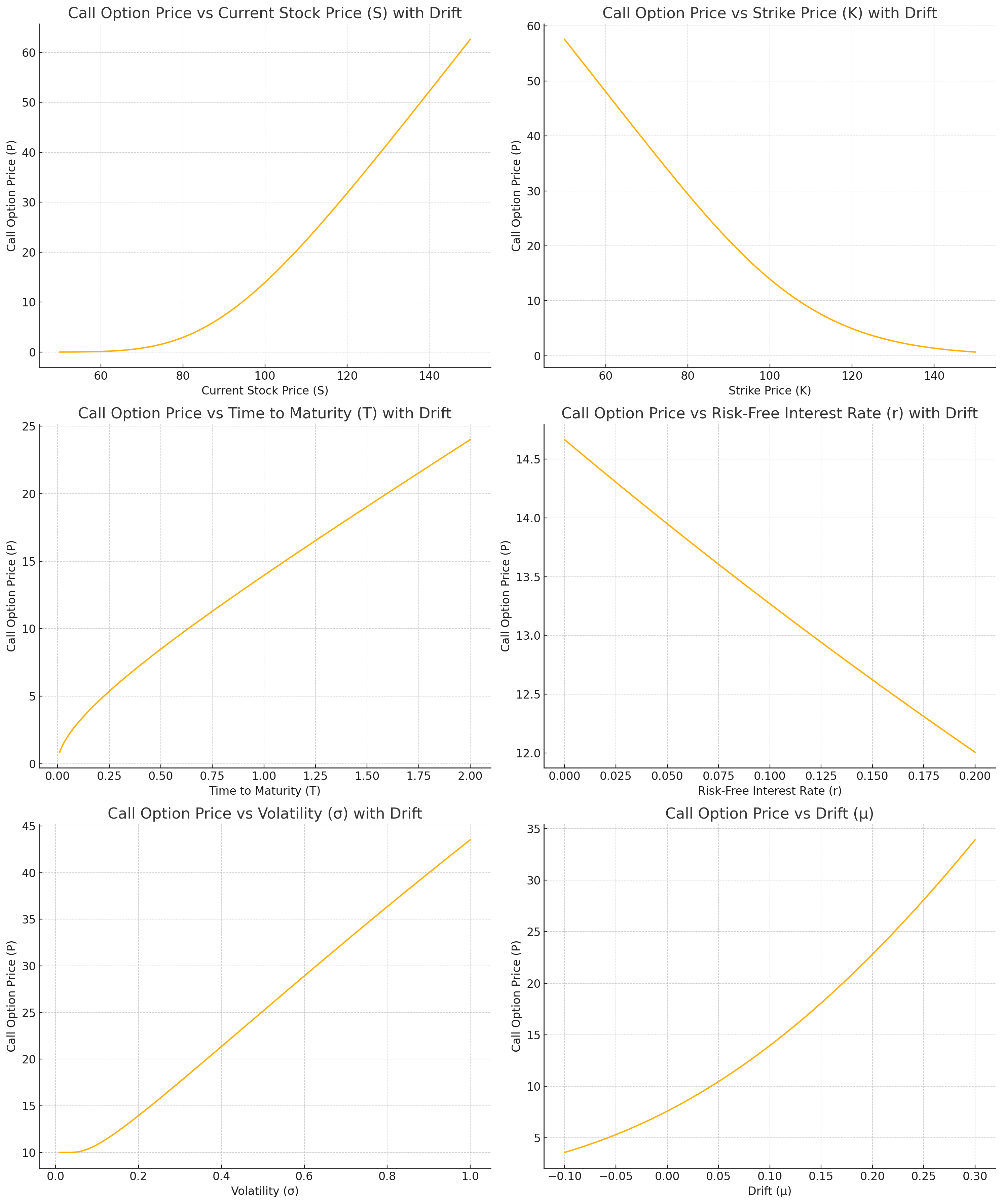
Fig. 16.2 Dependencies of a call option premium for a risk neutral investor, derived as the maximum premium the investor is willing to pay (reservation or indifference price). We use the parameters \(S_t=100\), \(K =100\), \(T-t = 1\) in years, \(r = 0.05\), \(\mu = 0.1\), \(\sigma = 0.2\).#
16.3.2. The arbitrage-free theory of derivatives pricing#
When we were applying the utility indifference theory of derivatives pricing to both parties agreeing in the transaction, the investor and the dealer, we found the issue that according to this theory, there would be a trade only if both of them are risk averse, since they are taking opposite sides of the bet on the payoff result. In reality, both dealers are investors are generally risk-averse and we observe transactions, so what are we missing in our theory?
The answer, as we anticipated above, is that the dealer is not really simply taking the opposite of the bet. There are mainly two ways a dealer will conduct this business:
If the market on derivatives is relatively liquid in both sides, with plenty of investors willing to take the long or short position in the derivative over periods much shorter than the expiry, the dealer will act as a market-maker of the derivatives. In this case, the dealer will quote bid and asks prices for the derivatives that compensate it for the provision of liquidity with its own capital, incurring potential inventory risk or information asymmetry risk
If the market is one-sided and / or illiquid, in the sense of having a small number of potential transactions before the expiry of the contract, the dealer will try to hedge the risk using other financial instruments available.
In practice, a combination of both situations will also happen often
As we discussed in the first part of this chapter, if we are in the first situation, we might not need a derivatives pricing model since we can extract the prices of derivatives directly from observations of trades or request for quotes that are not closed. It is the second case where we need a theory of derivatives pricing that takes into account potential hedging strategies that mitigate the risk of the dealer. We anticipate then that in this framework, the minimum price or premium that the dealer will accept to sell the derivative will be one that compensates it for the costs of hedging plus the residual risk.
More interestingly, we will see that in some cases, under certain theoretical situations, a perfect hedging strategy might exist, so the minimum price will be exactly the cost of the hedging strategy, which in this setup is also called the perfect replication strategy (since a perfect hedging implies no risk, and therefore a replication of the payoff using other financial instruments). A consequence of the existence of such replication strategy is that dealers are forced to price derivatives consistently, otherwise they would be generating risk-free arbitrage opportunities where other dealers who price correctly the derivative trade with the one miss-pricing it, and pocket the difference without risk. Hence, this theory of derivatives pricing is also called the arbitrage-free theory of derivatives pricing.
Let us revisit the case of forwards and options under this optic.
16.3.2.1. Example: Forward on a non-dividend paying stock#
Under the modelling hypothesis used in the previous sections to value the premium of a forward, namely, that 1) the interest risk is locked during the period of the forward, 2) there is no counter-party risk, i.e. no risk that the investor will not satisfy its obligations, then there is actually a simple replication strategy that hedges all the risk of the contract. If the dealer is selling the forward to the investor, therefore guaranteeing a price \(K\) to buy a share at time \(T\), then:
Borrows \(S_t\) dollars in the repo monetary markets at interest rate \(r\) during the period of the forward. We assume that interest accrues daily but is settled at the expiry. The stock bought is used as collateral in the repo.
Buys the underlying stock with this money at inception, paying \(S_t\)
At the expiry of the forward it delivers the stock to the investor, receives \(K\) and repays the loan plus remaining interests
If we consider that daily accruing of interest can be well approximated by continuous accruing, then the investor needs to repay at \(T\) an amount \(S_t e^{r(T-t)}\). The payoff for the dealer at the expiry is therefore:
which is deterministic under the hypotheses of the model. A rational dealer of course will not accept a determinist loss, so the minimum premium that will command for this contract is the discounted value of this payoff:
In practice, forward markets work by quoting the strike such that the premium is zero, hence:
This is the arbitrage-free price of a forward contract. As mentioned above, it is called arbitrage-free since any other price would represent a risk-free arbitrage opportunity for other dealer. For example, let’s assume this dealer quotes a \(\bar{K}_t < K_t\). Another dealer could buy the forward from the dealer, and use the opposite replication strategy:
Borrow the stock in repo and sell it in the market at price \(S_t\) to fund the repo.
At time \(T\) close the repo with the stock delivered by the dealer selling the forward, receive \(S_t e^{r(T-t)}\) in cash and pay \(\bar{K}_t\).
The payoff for this dealer is then:
i.e. a risk-free profit!
16.3.2.2. Example: European Call Options#
In the case of options there is no such obvious static replication strategy if we are only allowed to use the underlying stock and repo contracts. By static replication strategy we mean that we don’t need to modify the positions of the replication portfolio (the stock and the repo) during the life of the forward. If we are able to trade other derivatives there is actually a static replication strategy. If the dealer sells the call option to an investor, then immediately
Buys to other dealer a put option with the same strike and expiry
Buys to another dealer a forward with the same strike and expiry
The payoff at the expiry is:
meaning that the replication portfolio of a put and a forward replicates the call option. At inception, the dealer is paid for the call a premium \(P_{C,t}\) and pays \(P_{P,t}\) for the put and \(P_{F,t}\) for the forward, hence the payoff at inception is:
In order to avoid losses, the minimum premium that must command is therefore:
which is called the put-call parity relationship. The premium for the forward can be derived as discussed in the previous section, however we are left with a sort of chicken and the egg problem with regards to the call and put premiums: given one, we can determine the other, but we don’t have yet a replication strategy for the put to derive the call premium, and vice-versa.
If no static replication is available, is it possible to find a dynamical one that reproduces the payoff without uncertainty? Or are we left with strategies that, though they might minimize uncertainty, they don’t remove it and therefore we need to go back to our utility indifference theory?
16.3.2.3. The Black - Scholes - Merton Model#
Fisher Black and Myron Scholes [@black1973pricing], and separately Robert Merton [@merton1973theory] provided an answer to this question: under certain theoretical conditions, we can indeed find a dynamic replication strategy based on the underlying stock and a risk free account, that reproduces the payoff with no uncertainty. The main conditions are the following:
The stock price follows a Geometric Brownian Motion dynamics:
The replicating portfolio is composed of a position \(\Delta_t\) in the underlying stock and a cash account \(\beta_t\) from which we can borrow or lend money freely at a determinist risk-free rate \(r\):
The position in the stock can be adjusted continuously over the life of the option, without restriction like market trading hours, etc. There are also no transaction costs when buying or selling the stock. There are no restrictions on shorting the stock.
The replication portfolio is self-financing, meaning that no cash is added or withdrawn from the portfolio after the initial investment. Any proceeds from selling at immediately reinvested in the portfolio. Mathematically, it means that:
There is no counterparty default risk, i.e. the investor and the dealer will pay whatever obligations they have at the end of the option
If the portfolio \(\Pi_t\) indeed replicates the option payoff at the maturity \(T\) in any scenario, we must have \(\Pi_T = C_T = (S_T - K)^+\), where we have considered a Call option but the argument applies to any other payoff function. But since by construction the portfolio \(\Pi_t\) is self-financing, then if such dynamic strategy exists we must have \(\Pi_t = C_t\) for any time \(t \leq T\). Otherwise, there would be a risk-free arbitrage opportunity, e.g. selling the option at price \(C_t\) in the case \(C_t > \Pi_t\), buying with the cash from the premium the replicating portfolio \(\Pi_t\) and making an instantaneous gain of the difference \(C_t - \Pi_t\). The same reasoning applies \(C_t < \Pi_t\), only in this case we buy the option paying a discounted premium. Therefore, if we can find such strategy we immediately solve the problem of option pricing, since the premium is equal to the cost of replication by using the non-arbitrage opportunity argument.
The condition \(\Pi_t = C_t\) is equivalent to \(\Pi_T = C_T\) and \(d \Pi_t = dC_t\). Additionally, this equality implies that \(C_t = C(t, S_t)\), i.e. the premium of the option has to be a function of time and the contemporary value of the stock. We can then use Ito’s lemma to further understand the requirements for such strategy to exist:
Grouping the terms dependent on \(dt\) and \(d S_t\) separately we have:
Since the equality must apply for any arbitrary \(dt\) and \(dS_t\), each term in parenthesis must cancel separately. Starting with the right hand term we have:
which is call the delta-hedging condition, given its obvious connection with linear hedging strategies where we try to neutralize the exposure of a financial portfolio to a risk factor like the stock price in this case. Delta hedging the portfolio we ensure that its value is independent on the random dynamics of the stock, at least during an infinitesimal time. However, a strategy that delta-hedges at every time the portfolio is not necessarily self-financing, i.e. we might need to add extra cash during the life of the portfolio. The problem is that a priori the cash required for delta-hedging would depend on the path of the stock, making it a random variable. In that case the premium would also be a random quantity with a certain distribution.
In order to have a deterministic premium the portfolio has to be self-financing, which requires that the first term of the equality above is also zero, namely:
where we have used the self-financing condition \(\beta_t = \Pi_t - \Delta_t S_t = C_t - \frac{\partial C_t}{\partial S_t} S_t\). The resulting equation is the celebrated Black-Scholes-Merton (BSM) partial differential equation. Solving this equation with the terminal condition \(C_T = (S_T - K)^+\) allows us to compute the value of the premium for any time \(t \leq T\) deterministically. Therefore, by virtue of the replicating portfolio and non-arbitrage opportunity arguments, if the Black-Scholes-Merton conditions are satisfied the price of an option is no longer a random quantity as in the utility indifference framework.
Before discussing the solution to this equation, we can get another insight simply by inspecting it: the option premium does not depend on the drift \(\mu\) of the stock, only the volatility. In the utility indifference framework, the estimation of the drift plays a big role in the price that the investor is willing to pay for the option, since it affects the probability of exercising or not the option. However, for a dealer pricing the option, as far as the BSM framework holds, the directionality of the market is irrelevant since the strategy guarantees a replication of the payoff in any scenario by investing the premium into the BSM dynamic portfolio and implementing the dynamic strategy.
16.3.2.4. Solving the Black-Scholes-Merton equation#
There are different ways to solve the BSM equation. Most introductory textbooks on the topic (see for example [@joshi2003concepts], [@wilmott2007introduces]) follow the derivation used in the seminal paper that uses an ansatz for the solution that transforms the equation into the heat-equation, whose analytical solution is well-known [@evans2010partial]. Here, we will take a different approach and use the Feynman - Kac theorem introduced in Chapter (#stochastic_calculus), section (#feynman_kac). Recall that the Feynman - Kac theorem provides a general solution to a family of partial differential equations in term of an expected value. In the interest of the reader we review it again here: the solution to the PDE
with the boundary condition \(u(x,T) = f(x)\), is the following expected value
where \(X_t\) satisfies the general stochastic differential equation:
The BSM equation is a specific case of this general PDE where \(X_t \rightarrow S_t\), \(u(x,t) \rightarrow C(s, t)\), \(\mu(x,t) \rightarrow r\), \(\sigma(x,t) \rightarrow \sigma\), \(r(x,t) \rightarrow r\). The solution of the BSM equation can be expressed as:
where \(S_t\) satisfies the SDE:
The first crucial observation is that the solution is remarkably close to the one analyzed in the context of utility indifference pricing for a risk-neutral investor, with one caveat: the expected value is taken with respect to a SDE for the stock price that has the drift \(\mu\) replaced by the risk-free interest \(r\). In the former, the investor was taking the risk of the contract, but was indifferent to risk. In the latter, the dealer might be risk averse, but since the BSM dynamic hedging strategy neutralizes the risk (if the hypotheses are correct), there is no risk taken, only a deterministic cost to execute the hedging strategy, which is charged to the investor as the premium (plus potentially a margin for the service). In the jargon, the dealer prices the derivative as a risk-neutral investor if it computes probabilities in a different probability measure, where the drift is \(r\). Such measure is usually called the risk-neutral measure. This framework for derivatives pricing can be generalized to other derivatives, allowing dealers to compute prices directly skipping the construction of the hedging portfolio and solving the PDE. It is appropriately referred as risk-neutral derivatives pricing.
From a financial point of view, though, it is convenient not to lose the connection to the dynamic hedging strategy, since the validity of this theory is linked to the validity of the hypotheses done to derive the PDE. If we are interested in introducing more realistic dynamics into the pricing, like non-continuous hedging and transaction costs, we need to start again from the point of view of the replication portfolio and the hedging strategy. When those hypotheses are relaxed, though, we come back to a probability distribution to characterize the premium of the option instead of a deterministic one, the latter being one of the main remarkable results of the BSM theory.
The computation of the expectation value for the option premium can be reused from the one done in the context of utility indifference pricing, simply by substituting \(\mu \rightarrow r\) in the expressions:
where:
This is the infamous Black-Scholes-Merton option pricing formula. It provides dealers with option prices that depend on
the current stock price \(S_t\)
the expected volatility of the stock \(\sigma\)
the risk-free interest rate \(r\)
the time to maturity \(T-t\)
the option strike \(K\).
It does not depend on the stock drift \(\mu\), i.e. the expected trend of the market. This is because in the BSM framework, the dealer uses the dynamic hedging strategy to make the portfolio risk-free and therefore shielded from any market trend.
Again, we must emphasize that despite the similarity with the risk-neutral option premium computed in the utility indifference framework, in the BSM framework the dealer is not computing the premium based on real probability scenarios of stock prices. The connection between replicating strategies and expectation values provided by the Feynman - Kac theorem is a useful mathematical result that simplifies the computation of derivatives premia in the BSM framework. But they shall not be interpreted in the sense of real probabilities (or probabilities in the real probability measure, as they are also referred to).
The dependencies of the option formula for a European call option with respect to the parameters are similar to the ones seen in the context of utility indifference pricing, with the exception of the dependence with respect to the risk-free interest rate \(r\), whose role in the formula goes now beyond cash-flow discounting. In the following picture we compare the premia derived with BSM versus utility indifference pricing:
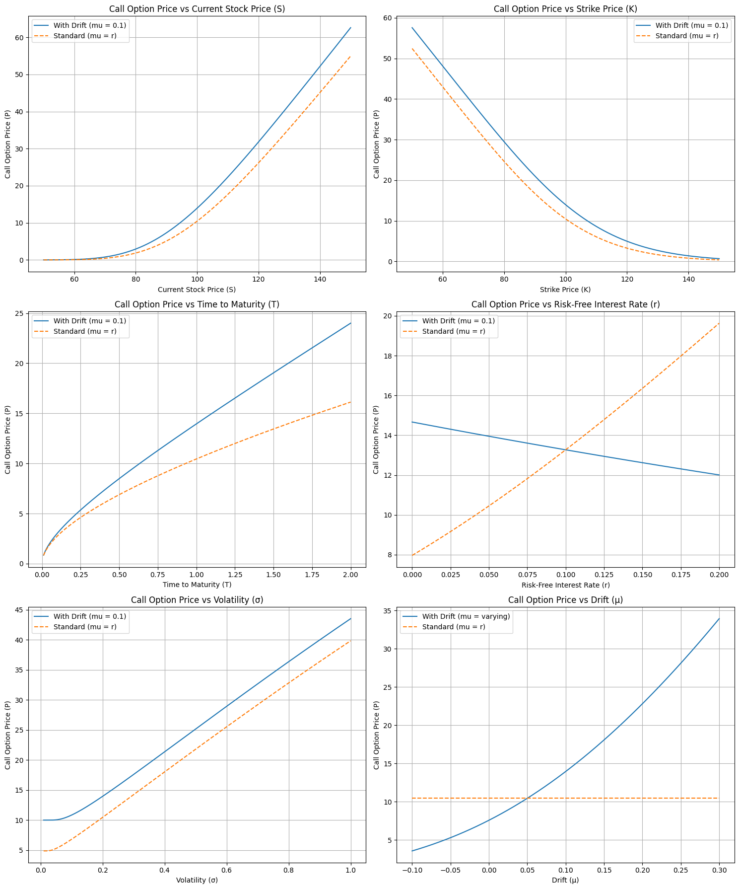
Fig. 16.3 Option price premium calculated using the utility indifference pricing versus arbitrage-free theory. The results are shown for an european call option with parameters \(S_t=100\), \(K =100\), \(T-t = 1\) in years, \(r = 0.05\), \(\mu = 0.1\), \(\sigma = 0.2\).#
The first main differences is, as commented, the dependence with respect to the risk-free interest: in BSM theory, the premium is more valuable as interest rates increase, wheres in utility indifference pricing it was the other way around. In the latter, interest rates enter the formula to discount the value of future cash-flows. As interest rates grow, the opportunity cost of investing the premium for the future cash-flows of the options increases, since a risk-free deposit generates comparatively a larger yield. In other words, for an investor, the option becomes less attractive and is willing to pay less for it. However, in BSM theory used by dealers to price options, the opposite happens: bigger interest rates make funding the hedging strategy more costly, therefore requiring a larger compensation in terms of premium to execute the replication strategy.
The second big difference is of course the dependence with respect to the expected market drift, since in the BSM theory the premium is independent of it. The resulting plot is interesting because it points out to the resolution of the question of why are options traded in practice, assuming both dealers and investors have the same view of the market. As mentioned before, if both were to value the option as an investment, there would be no agreement on the premium to pay, since they hold opposite sides in the trade. However, if the dealer uses BSM theory there is room for agreement, at least for those investors whose expectations on market drifts make the premium requested by the dealer attractive. In the picture, such situation corresponds to those expected drifts that make the premium that an investor is willing to pay larger than the one commanded by the dealer.
From a classical Economics point of view, those frameworks fit well together to explain the derivatives market in terms of demand and supply. Demand for options is driven by investors looking to generate returns on investment, whereas supply comes from dealers that “fabricate” those options using replication strategies. The BSM premium is essentially the cost of “fabricating” the option, in analogy to the language used in the production of goods.
16.3.2.5. An alternative derivation: the market price of risk#
An alternative derivation of the BSM equation that can be helpful to gain intuition on the theory uses the financial concept of market price of risk. The market price of risk is essentially a Sharpe ratio, commonly used in the theory of investment. The Sharpe ratio computes the excess returns of an investment, i.e. the expected returns devoted fom the risk-free interest, over their risk defined as the volatility of the returns. For the stock that is the underlying of the option, and using continuos time, this is:
CHECK AND CITE REBONATO
We can now use Ito’s formula to compute the market price of risk of the option:
We can now apply a different version of the arbitrage-free theory. Since the value of the option is essentially derived from the underlying stock, which the only risk factor affecting the option price in the BSM theory, then as investment opportunities both should have the same Sharpe ratio or market price of risk, i.e. \(\lambda_S = \lambda_C\). Otherwise, investors would bid up the price of the one with the largest Sharpe ratio until both of them equalize. Applying this equality the terms proportional to the drift \(\mu_t\) cancel and we get back to the BSM differential equation.
One could of course have used the argument in reverse, reorganizing the BSM equation in terms of market prices of risk to prove that the equality of those is a consequence of the arbitrate-free argument used when building the replication portfolio.
16.3.2.6. Using the BSM framework in practice#
The Black - Scholes - Merton pricing theory supposed a change of paradigm for dealers creating liquidity in option markets. The theory allows for a consistent pricing of derivatives beyond options, providing not only a way to calculate the premium but a hedging strategy that neutralizes the risk of the derivative, or from a different angle, a recipe to synthesize those derivatives from liquid tradable instruments.
However, the BSM theory is based on multiple hypothesis that are not necessarily realistic, so the dealer needs to take into account how relevant is for the pricing and hedging of derivatives that those hypothesis are not consistent with reality. For instance:
The BSM theory does not take into account liquidity and transaction costs of the hedging instruments, which will increase the costs of the replication strategy in a non-deterministic way. The premium becomes dependent on specific market microstructure details of how the instruments of the hedging portfolio are traded, for instance if they are traded in limit order book based markets, the fees of orders, the bid-ask spread, the tick size, etc. How the dealer executes those trades becomes also relevant, for instance, which types or orders are used, or if execution algorithms are to be used, in whose case the theory needs to incorporate an estimation of the cost of execution of those strategies, based on transaction cost analysis (TCA)
The BSM theory assumes continuous hedging, which is not feasible in practice, both because of the costs mentioned in the previous point, and because markets in financial instruments usually are not open 24 hours per day. Even when they do, liquidity tends to vary widely across trading hours. In practice, dealers tend to hedge less frequently (e.g. daily), deviating from the pure BSM paradigm
The BSM theory assumes a specific dynamics for the evolution of the underlyings, namely the Geometric Brownian Motion in the case of stocks (for underlyings that can become negative, like interest rates or inflation, a Brownian Motion is also typically used). Markets in practice follow more complicated dynamics, for instance they exhibit fatter tails in the distribution of returns or they might show sudden jumps, particularly in the overnight gap [2].
The original BSM theory assumes hedging strategies based on the underlying. The theory can be applied equally if we assume hedging with other derivatives as far as they share the same underlyings, or in a more fundamental level, the same risk factors driving the underlyings. In practice, dealers might use liquid derivatives to hedge non-liquid ones. For instance, european options with non-standard strikes or maturities with respect to liquid ones traded in exchanges. As an exercise for the reader, we propose to prove that the Black-Scholes-Merton differential equation can be derived using a hedging portfolio where instead of the underlying we trade another option with a different strike.
In general, these deviations from the assumptions make the premium no longer deterministic, since they introduce uncertainty in its estimation. Dealers typically will need to estimate how much do they need to increase the BSM premium to compensate for those risks. In the following plots we show the histogram of differences between the replication portfolio and the option payoff at maturity, when different assumptions of Black - Scholes - Merton theory are violated, namely:
Continuous re-hedging, which can be violated by using increasingly smaller frequencies of re-hedging
BSM volatility (the one used in the BSM pricing and hedging formulae) equals to market realized volatility
Lognormal stock dynamics, which can be challenged using a different dynamics like for instance the Heston model, which considers that volatility of the log-normal process is also stochastic, with its variance (volatility squared) following a CIR mean-reverting process:
Zero transaction costs, which can be violated for instance by assuming the dealer pays the half bid-ask spread of the market every time the underlying is bought or sold when rebalancing the portfolio.
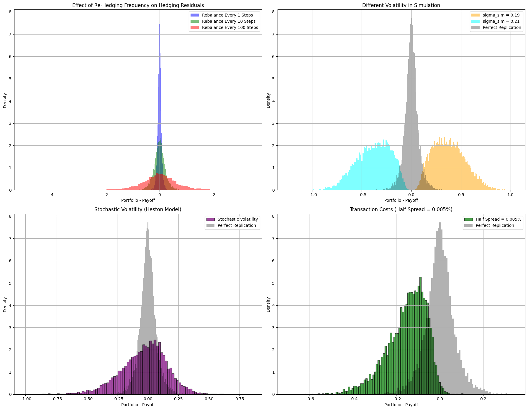
Fig. 16.4 Histograms showing the difference between the replication portfolio using the BSM dynamic hedging strategy, and the actual payoff of an European call option. Each plot shows the impact of violating a different hypothesis of the BSM theory. We run 10000 simulations for each case. We use the parameters \(S_t=100\), \(K =100\), \(T-t = 1\) in years, \(r = 0.05\), \(\mu = 0.1\), \(\sigma = 0.2\) for the baseline scenario where we expect close to perfect replication when re-hedging continuously. To test the effect of different realized volatilities we use use \(\sigma = 0.19\) and \(\sigma = 0.21\), respectively. To test the effect of transaction cost we add a constant bid-ask half-spread of 0.005%. To test the effect of a different market dynamics we use a Heston model with parameters \(\kappa = 20\) (mean reversion rate of the volatility squared), \(\theta = 0.04\) (long-term volatility squared mean), \(\xi = 0.2\) (volatility of volatility squared), \(\rho = -0.7\) (correlation between stock and stochastic volatility risk factors).#
In the plots, we can see the different impacts that the violations produce on the distribution of the residuals. Whereas a less frequent re-hedging increases the dispersion of the residual, those are still unbiased and symmetrical. Other violations produce skewed distributions with non-zero mean. When introducing transaction costs, residuals have a negative mean, meaning that the BSM premium is insufficient to cover the actual costs of replication, as expected since the BSM derivation does not take into account such transaction costs. The effect of a different dynamics for the underlying is more nuanced: depending on the actual process, the distribution of residuals might have positive or negative mean, meaning that the BSM premium over-estimates or under-estimates, respectively, the costs of replication. For instance, if the realized volatility is lower than the one used for pricing and hedging in the BSM model, the mean of the residual is positive. This is, again, intuitive, since as we seen the premium of the option increases with volatility, so overestimating it means charging a larger premium than necessary for replication. Notice that this is not necessarily good for a dealer in competition, since if other dealers have a better estimation of market volatilities, they will be able to offer more competitive prices to clients and close more deals.
16.4. Exercises#
Derive the Black-Scholes-Merton differential equation by using the portfolio replication argument for a dealer that hedges the risk of an european option (call or put) with strike \(K_1\) and maturity \(T\), using another (liquid) option tradable in the market with strike \(K_2\) and same maturity \(T\). As in the original BSM derivation, the dealer uses a cash account to remunerate cash positions or borrow cash. Formally, the replication or hedging portfolio is \(\Pi_t = \Delta_t C_2(S_t, t) + \beta_t\), with the terminal condition \(\Pi_T = C_1(S_T, T)\). Hint: link the result with the market price of risk for options introduced in this chapter.