18. Modelling RfQs in Dealer to Client Markets#
18.1. Introduction#
In the context of platforms where the client identity is known, like Dealer to Client platforms, the analysis of the client patterns of trading is relevant in order to fine-tune pricing and hedging models, or to optime the management of axes.
18.2. Probabilistic graphical model for RfQs#
A model that captures the Request for Quote process discussed in the Market Microstructure chapter is the probabilistic graphical model proposed by [11], which we reproduce in the following figure:
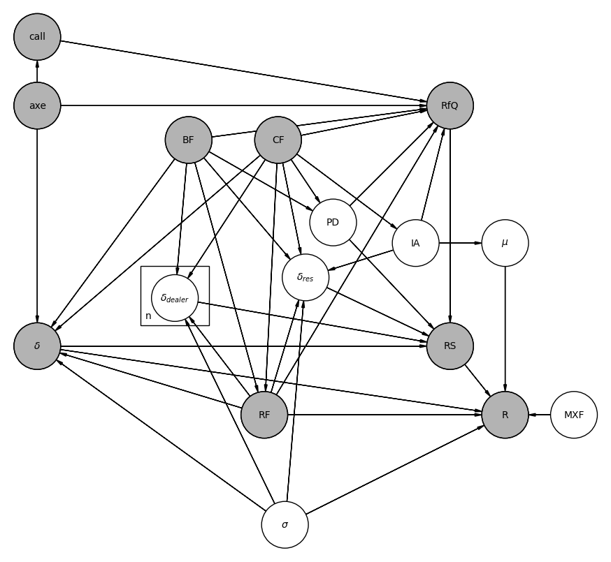
Fig. 18.1 Probabilistic graphical model for the Request for Quote process#
The model is composed of the following elements. Some of them are known pre-trade, others post-trade depending on the result of the RfQ, and some are just simply non-observable (latent) variables:
RfQ: a binary random variable indicating whether an RfQ is initiated. Each RfQ carries associated features, collectively represented by the variable RF in the model. These include, for example, the time \(t\) of the request, the side \(s\) (buy or sell) — where “buy” implies the dealer purchases from the client, and “sell” implies the dealer sells to the client — the volume \(v\), and the number of competing dealers \(n\) chosen by the client (typically subject to platform-imposed limits). The trigger for an RfQ can stem from external client factors, such as a specific trading strategy, which fall outside the model’s scope. In some cases, it may also result from proactive engagement by the dealer’s sales force, captured in the variable call. Other factors that may shape the client’s decision to request a quote, and which are explicitly included in the model, include:
Price discovery (PD): The client is interested in discovering the fair value of the instrument but has no intention to execute a trade. This intent is unobservable (a latent variable), as the dealer cannot infer the client’s true motivation at the time the RfQ is received.
Client information asymmetry (IA): If the client possesses meaningful information about the short-term direction of the market, this creates a situation of information asymmetry. There are several possible sources for this asymmetry:
The client’s trading activity itself may generate market impact, yet the RfQ submitted to the dealer often reflects only a portion of the total intended order. In this case, the information will affect the market and is captured in the model as a price drift (\(\mu\)) variable, with a direct link represented as \(IA \rightarrow \mu\).
Alternatively, the client might have access to insider information or sophisticated analytics that provide insight into future price movements. This scenario is also modeled via the drift variable, though here there is no direct causal connection between information asymmetry and drift —rather, the client forms an estimate of the drift but does not influence its true value post-trade.
Axe: A publicly expressed interest by the dealer in executing a trade at a favorable price (either bid or ask), which can increase the likelihood that a client will submit an RfQ.
Client Features (CF): Includes the identity of the client as well as broader attributes that may influence trading behavior—such as industry sector, geographic location, or credit rating.
Bond Features (BF): Encompasses the bond’s unique identifier along with its financial attributes—such as coupon, yield, maturity, and interest rate sensitivity (e.g., DV01). It also includes factors related to liquidity, such as market bid-ask spreads, volatility, and the typical number of dealers quoting RfQs in that bond.
RfQ Status (RS): The final outcome of the RfQ can be categorized into three main cases:
Hit: The client executes a trade with the dealer.
Missed: The client trades with a different dealer.
Passed: The client does not trade with any dealer. This may occur because the quotes were not attractive enough or the client was merely seeking price information (price discovery).
The drivers of the RfQ status in this model include:
The client’s intent to trade, which is what initiates a Request for Quote (RfQ) via a multi-dealer-to-client platform.
If the quote is requested solely for price discovery (PD) purposes, the only possible outcome with non-zero probability is a passed status (i.e., the client walks away without trading).
The half-spread (\(\delta\)) quoted by the dealer. Although dealers provide price quotes to clients, we assume that the client’s trading decision depends on the quoted spread relative to a reference mid-price \(P_{m}\). For example, using a composite price from the platform, the transaction price is modeled as:
\(P = P_{m} + s \delta\), where \(s = 1\) if the dealer is selling (ask), and \(s = -1\) if buying (bid).The spreads quoted by competing dealers, denoted \(\delta_{dealer}\). Clients may choose to include up to \(n\) dealers in the RfQ. Naturally, as \(n\) increases, so does the probability of receiving a more competitive quote. Typically, all quoting dealers know the number of participants \(n\), but not the individual prices submitted by others. The only partial post-trade information available comes when a dealer wins the RfQ and the platform discloses the cover price (i.e., the second-best price). The dealer who submitted this cover price is informed of their status as covered, but they do not receive information on the actual winning price.
The client’s reservation spread \(\delta_{res}\): the maximum acceptable spread relative to the mid-price, defined as
\(\delta_{res} = s(P_{res} - P_{m})\),
where \(s\) is the trade side as defined earlier.
If all quoted prices exceed this threshold, the client will not trade (passed status). Since \(\delta_{res}\) is not directly observable, it must be inferred from historical client behavior. Its determinants include client features (\(CF\)), bond features (\(BF\)), and RfQ characteristics (\(RF\)). Additionally, information asymmetry (\(IA\)) is expected to play a role—clients with better information may be more inclined to accept trades.
Likewise, higher market volatility (\(\sigma\)) may prompt clients to trade more readily (e.g., to reduce risk exposure).
Revenue (R): The profitability of the trade. Dealers use several different revenue metrics depending on the context:
Instantaneous Flow Value (\(R_0\)): A simple per-trade measure of profitability, calculated as \(R_0 = v \delta\) where \(v\) is the trade volume and \(\delta\) is the half-spread at the time of the trade. This metric does not consider the gains or losses realized when the inventory is eventually unwound via an opposite trade.
Round-Trip Revenue (\(R_{rt}\)): Addresses the limitations of the instantaneous flow value by considering the full round-trip (buy and sell or vice versa). Revenue is computed as:
\(R_{rt} = s v (P_{t_{rt}} - P_t) = v \delta_{t_{rt}} - v \delta_{t} + s v (P_{m,t_{rt}} - P_{m,t})\)
where \(t\) is the RfQ time and \(t_{rt}\) is the round-trip time.
Assuming Brownian motion for price dynamics:\(P_{m,t_{rt}} - P_{m,t} = \mu(t_{rt} - t) + \sigma (W_{t_{rt}} - W_t)\)
where \(\mu\) is the drift, \(\sigma\) is the volatility, and \(W_t\) is a Wiener process such that \(W_{t_{rt}} - W_t \sim N(0, t_{rt} - t)\) The stochastic component (\(W\)) captures the effect of market external factors (MXF). The model also allows for a causal relationship between information asymmetry (IA) and drift (\(\mu\)), to reflect situations where client trading influences market direction. Both \(\mu\) and \(\sigma\) are latent variables—not observable at trade time. However, the model assumes that \(\sigma\) (volatility) is relatively predictable, so its pre- and post-trade values are treated as equivalent. This makes it a valid driver of both dealer pricing (\(\delta\), \(\delta_{\text{dealer}}\)) and client reservation spreads (\(\delta_{\text{res}}\)). In contrast, \(\mu\) (drift) is much harder to predict reliably, except in cases where clients have asymmetric information. Hence, post-trade drift is excluded from dealer pricing logic.
End-of-Day Flow Value (\(R_{\text{eod}}\)): Used when trades remain open over long time horizons (e.g., illiquid bonds). Revenue is marked-to-market at the end of the day:
\(R_{\text{eod}} = v \delta_t + s v (P_{m,T} - P_{m,t})\)
where \(T\) is the end-of-day timestamp. This measure can incorporate liquidity penalties to reflect the risk of holding hard-to-sell positions.
Short-Term Flow Value (\(R_{t+h}\)): Evaluates revenue at a short time horizon \(h\) (seconds to minutes) after trade execution:
\(R_{t+h} = v \delta_t + s v (P_{m,t+h} - P_{m,t})\) .
This is particularly useful for identifying information asymmetry (IA), as such informational advantages typically manifest within short timeframes before being diluted by general market dynamics (MXF).
18.3. Generative models for the request for quote activity#
18.3.1. Models for the arrival of RfQs#
A dealer receives RfQs for different products from different clients every day or week. Each RfQ has a side, buy or sell, and a volume requested to be traded. A generative model that captures this distribution can be encoded by the following probability:
where \(\tau_{\text{RfQ}(\text{c, p, s, v})}\) is a random variable that specifies the time at which a client \(\text{c}\) requests a quote for product \(\text{p}\) of side \(\text{s}\) and volume \(\text{v}\) (for the moment we assume volumes to be discrete), and we have also a filtration \(F_t\) that includes all relevant information up to t. Alternatively we can introduce \(N_t^{\text{RfQ}(\text{c, p, s, v)}}\) as the number of such RfQs up to time t. These two formulations are in fact equivalent:
From the Stochastic Calculus chapter we recognize this model as a counting process, whose probability distribution we can write as:
with the so-called intensity \(\lambda_t\) being a general function of time, RfQ variables and any relevant information contained in \(F_t\), for instance, previous RfQs. This is an instance of a non-homogeneous Poisson process. If it also depends on previous times of arrivals of RfQs, i.e. it is a self-exciting process, we have a Hawkes process. Such counting processes are natural candidates to model the arrival of RfQs.
Alternatively, we can rewrite the model using the product rule of probability as:
where we have used the compact notation: \(\text{RfQ}_{t,t+dt}\) instead of \(\tau_{\text{RfQ}} \in [t, t+dt]\). This way, we can explicitly model the statistics of each of the probabilities in the product. A typical hypothesis is to make the conditional probabilities independent of time and use simple distributions to model them. For instance, volumes are modelled in many cases as continuous distribution following a power law or a log-normal probability density, since volumes are positive and heavy tailed in their distribution:
where \(v \geq v_\text{min}\), \(\alpha > 1\).
The side \(s\), being a binary variable, buy or sell, is typically modelled using a Bernoulli distribution. Finally, the probabilities that RfQs come from a specific client or product can be modelled using a multinomial distribution.
18.3.2. Attrition risk#
The previous model considers that clients have a stable pattern of choosing the dealer for their requests for quotes. However, clients might at some point stop sending RfQs to the dealer, for instance when they perceive that prices are non competitive on average (i.e. they see low hit & miss ratios) or when dealers often don’t respond with their quotes.
A simple extension of the previous model for the arrival of RfQs introduces a latent binary random variable to characterize if clients are actively engaging with the dealer or not. Denoting this variable \(a\), with \(a=1\) meaning the client is active, the model is decomposed as:
where we have implicitly used the fact that \(P(\tau_{\text{RfQ}(\text{c, p, s, v)}} \in [t, t+dt]|a = 0, F_t) = 0\), i.e. we don’t expect the arrival of RfQs for clients that are inactive. We are therefore interested in characterizing \(P(a = 1|F_t)\) or most typically \(P(a = 0|F_t) = 1- P(a = 1|F_t)\), which is known in the marketing analytics literature as the attrition risk model.
Inferences of attrition risk can be done by analyzing the historical patterns of client trading activity. A simple albeit elegant model is that from Fader et al [12], where they consider daily (or any other time scale) client activity as a set of independent identically distributed Bernoulli random variables \(Y_t\) with probability \(p\). In our RfQ setup, this means \(Y_t = 1\) if the client sends any RfQ, or \(Y_t = 0\) otherwise. Additionally, a client can become inactive at the beginning of the day with probability \(\theta\). Given a pattern of historical daily activity \(D\) of a client we can compute the probability that the client is active using Bayes’ theorem:
For example, for the pattern \(D = 10100\), the likelihood in the denominator is calculated as the probability that the the observed pattern is simply explained by the natural probabilities of requesting RfQs:
with the prior probability for the client being active corresponding to the scenario in which the client does not become inactive in all the observation periods:
In contrast, the alternative hypothesis in which the client is already inactive is actually the result of two different paths, one in which the client becomes inactive at the last day, whereas in the second it does it in the previous day. Therefore:
The model does not consider the possibility that clients which are inactive are activated again, which is definitely possible in reality, but not necessarily useful for a model that simply tries to detect clients that have recently stopped engaging with the dealer. Plugging these probabilities into Bayes’ theorem we get:
As pointed out by the authors, any other trading pattern with the same number of active days –denoted as \(x\) (frequency in the marketing jargon), and the same number of days since the last RfQ –the recency \(r\), has the same likelihood. For instance, \(P(a = 1|D = 10100, p, \theta) = P(a = 1| D = 01100, p, \theta)\). see the exercise at the end of the chapter. This is an interesting insight that naturally links the model with the traditional heuristics based on recency and frequency in the Marketing Analytics literature, see for example [13]. The general result for a pattern consisting of \(n\) days of trading activity, frequency \(x\) and recency \(r\), we have:
Notice that the evidence in the denominator of Bayes’ theorem it is simply the complete likelihood of the data:
Therefore:
The model in this form requires a separate estimation of parameters \(p\), \(\theta\) for each individual client. Alternatively, the model can be generalized to a segment of clients whose parameters follow a probability distribution but we cannot attach specific parameters to any of them. As it is natural to model distributions of probabilities, Fader et al propose the use of Beta distributions for \(p\) and \(\theta\):
where the Beta function is by definition:
This allow us to characterize the segment of clients with four parameters, \(\alpha\), \(\beta\), \(\gamma\) and \(\delta\). Notice that this model does not capture the possibility of multiple segments within the population of clients. To capture that, a simple extension is to use a mixture of Betas, see next section for a simple application of such model in anomaly detection.
Continuing with the single segment model, the likelihood now requires to integrate over the distribution of \(p\) and \(\theta\):
where recall that in this model, the dataset \(D\) can be reduced to \(n\), \(r\) and \(x\). The calculation can be carried out analytically in terms of Beta functions, since it involves integrals of the form:
The likelihood for a single client can be expressed in terms of Beta functions:
Applying accordingly Bayes theorem on \(P(a = 1|D, \alpha, \beta, \gamma, \delta)\) we get:
where we have defined \(L(D|\alpha, \beta, \gamma, \delta) \equiv P(D|\alpha, \beta, \gamma, \delta)\)
For model parameters estimation, the authors suggests using maximum likelihood over the historical dataset. For the one segment model this implies a joint estimation of the parameters for the collective of clients in the dataset, since they share parameters. Alternatively, a Bayesian estimation approach would seek to estimate \(P(p, \theta|D)\) for the single client model or \(P(\alpha, \beta, \gamma, \delta|D_N)\) for the one segment model, where we have used \(D_N\) to denote the full dataset of \(N\) clients.
18.3.2.1. Simulation of attrition risk#
Let us see how this model works in practice. We simulate a segment of 50 clients that send RfQs to a dealer according to the Poisson model discussed in the previous section. For simplicity, we only consider the situation in which the client wants to buy from the dealer. Each client is characterized by an intensity of RfQ arrival drawn from a Gaussian distribution with mean 1 (i.e. a client on average sends one RfQ per day) and standard deviation 0.05. In principle such choice of parameters makes highly unlikely to generate negative intensities, but if that happens we simply force them to be positive. The clients’ reservation prices, i.e. the maximum prices they would accept in order to trade, also follows a Gaussian distribution, in this case with mean 100 (which could be considered the fair price of the financial product) and standard deviation of 10% around this mean. These reservation prices are not static, though: they fluctuate over time with some noise that models the potential impact of changing market conditions. We choose 20% of the mean for this parameter.
We model attrition in this setup by considering that clients will stop sending RfQs to the dealer if the average hit rate (percentage ot trades over RfQs sent) is below a given threshold over a window of time. We take 10% as the threshold for all clients (although we could also model a distribution over the segment) and suppose that clients evaluate the hit rate with the dealer over a 10 days window (again, this could be made client dependent but we choose not to in this simulation).
Finally, in order to produce a rich dynamics, we model the behavior of the dealer as follows: on the one hand, she has her own target hit ratio that tries to balance client satisfaction with he own profitability. We choose a 40% hit ratio target for all clients. To hit this target, the dealer try to infer the distribution of each of her clients’ reservation price using Bayesian methods, i.e. estimating the posterior distribution of the reservation price conditioned to the data, which consist of the time series of hits and misses of previous RfQs sent by clients and the prices quoted. Mathematically, let \(r_n\) the reservation price of client \(n\), then the dealer seeks to infer the density function \(f(r_n|D)\), where \(D = \{(c_i, p_{i}, h_{i})\}\) is the dataset comprised of clients \(c_i\), the prices \(p_{i,n}\) quoted to client \(n\), and the result of the negotiation \(h_{i,n} = (1,0)\) equal to one when the client accepts the price (hit) and zero otherwise (miss). The dealer updates the posterior dynamically after every negotiation, and uses this information to quote the next RfQ by choosing the price such that the probability of hit (which occurs when the price quoted is lower than the reservation price) is equal to the hit target of 40%:
At the beginning of the simulation, we assume that the dealer has a prior estimation of the distribution of reservation prices given by a Gaussian distribution of mean \(60\) and standard deviation \(10\), which means the estimation is relatively off with respect to reality.
Let us simulate the model over 200 days. The following figure shows the mean of daily hit ratios that the dealer achieves with the clients that send RfQs that day (which are active by definition, although there could be active clients that a given day don’t send RfQs):
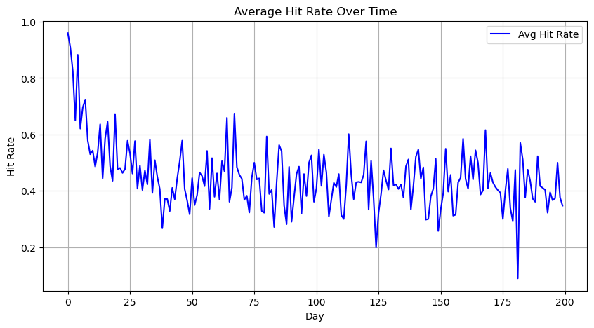
Fig. 18.2 Evolution of daily averages of hit rates with clients that sent RfQs each day. The dealer start with an off estimation of the reservation prices, which explains why it takes some time for dealers to reach their target hit ratios.#
The effect of the prior estimation of reservation prices by the dealer is clearly reflected in the first part of the simulation, where hit ratios are far from the target set by the dealer. In particular, since the dealer has a low biased estimation of reservation prices, this translates into high hit rates at the beginning of the simulation. We see the effect of the Bayesian learning, though, as time goes on, since in the range of 25-50 days the hit rates have stabilized around the target, which remains noisy given the fluctuations in client reservation prices that we have introduced in the model. Precisely because of these fluctuations we find situations in which clients get average hit rates over their 10 days evaluation windows below their 10% target, which makes them stop sending RfQs to the dealer –becoming inactive, although they don’t inform the dealer of this situation. The following figure reflects this situation by plotting the evolution of the attrition rate, i.e. the cumulative percentage of clients who have become inactive since the beginning of the simulation:
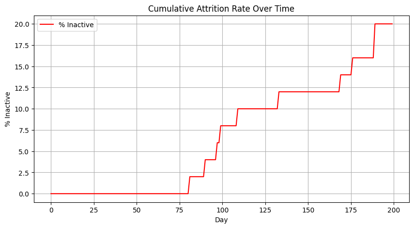
Fig. 18.3 Cumulative attrition rate over time, i.e. percentage of inactive clients over the total number of clients (50) at the beginning of the simulation.#
Precisely because the dealer starts with a pessimistic estimation of the reservation price of the clients, which translates into a large hit rate, attrition rates don’t kick off until the dealer corrects her estimation of the reservation prices and reaches her target hit rates. At this point, fluctuations in the reservation price from clients trigger attrition rates, which steadily grow over the simulation. If the dealer does not do anything to address the attrition risk, eventually all clients will become inactive. That’s where the attrition risk model comes into play, as a tool used by the dealer to detect which clients might have become inactive and trigger corrective actions, for example using her salesforce to contact clients and try to engage them back.
We implement the model discussed in this section based on the work by Fader et al and fit it using maximum likelihood over the first 100 days of the simulation. Then we use it to evaluate the probability of being inactive for each client in the last 100 days, given their trading patterns. To check that the model is well calibrated, we plot the expected attrition rate from the model against the simulated one in the test set (last 100 days) in the following figure:
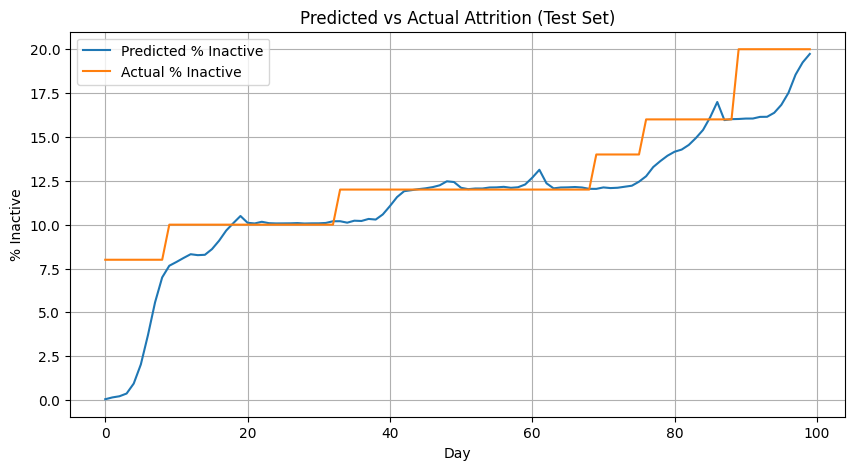
Fig. 18.4 Expected attrition rate computed by the model against the actual attrition rate from the simulation in the test set (the last 100 days of the simulation). The good match is an indication of a good calibration.#
The figure shows a good agreement between model and simulation in the test set, implying that the model is reasonably well estimated. We further test the quality of the model by computing a confusion matrix that compares the prediction of the model: inactive if the probability of attrition is higher than 50%, active otherwise; against the hidden activity labels we have generated in the simulation, where clients become inactive when average hit rates are lower than 10% for the last 10 days. This is evaluated for each day and client in the test set (5000 evaluations, resulting from 50 clients over 100 days).
The results indicate that the model is able to discriminate well between active and inactive clients across all thresholds, as evidenced by a high AUC of 0.9884. At the specific threshold of 50%, overall accuracy is very high (98.48%) and precision is perfect (100%), meaning that every client flagged as “inactive” truly was inactive. However, recall is 88.03%, which implies that the model misses some truly inactive clients (76 false negatives vs. 559 true positives). In practice, this means the model is conservative in raising alerts: it waits for clear evidence of non-trading before flagging a client, avoiding false positives entirely but potentially reacting slightly late. Depending on the cost a dealer might incur in missing early signs of disengagement, it may be worth exploring a lower threshold to catch more potential churn cases earlier, even if that introduces some false positives.
Finally, let us check the behavior of the model for individual clients over the test set, with selected clients shown in the following figure:
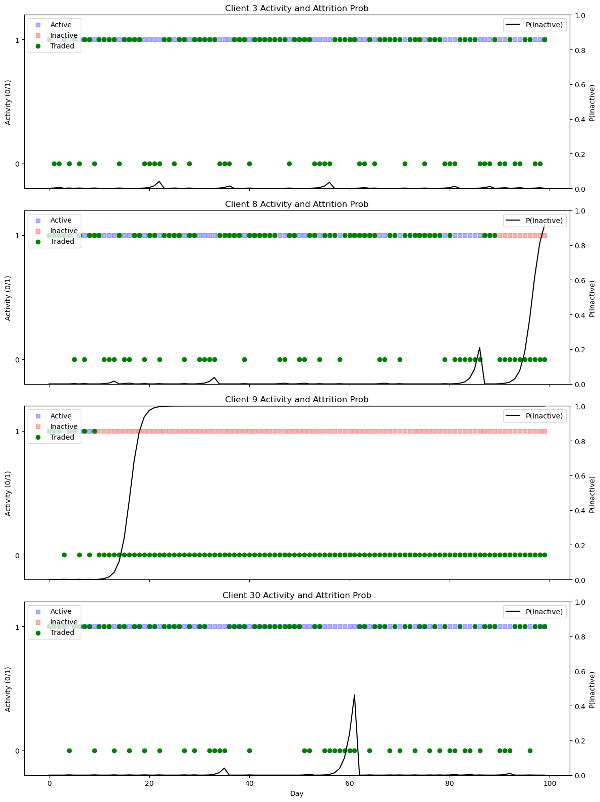
Fig. 18.5 Trading behavior and activity for selected clients, against the probability of being inactive (attrition risk) computed by the model.#
The visualizations of Clients 3, 8, 9, and 30 illustrate how the model responds to different trading behaviors over time with its attrition probability signal.
Client 3 remains consistently active throughout the period. Accordingly, the model keeps the attrition probability near zero, reflecting high confidence in continued engagement.
Client 8 begins active but stops trading near the end of the test period. The model gradually increases its attrition probability, reaching high levels just as the client becomes inactive. This indicates that the model correctly detects disengagement with a slight delay, requiring some sustained evidence of inactivity before triggering an alert.
Client 9 becomes inactive early (around day 15), stopping trading entirely. The attrition probability reacts sharply, climbing quickly toward 1 and staying there for the rest of the period. This is an ideal response, showing the model can detect early and persistent disengagement with high confidence.
Client 30 shows intermittent trading throughout, with a notable gap around day 60. During this gap, the model’s probability of inactivity rises significantly, but it drops again once trading resumes. This demonstrates the model’s sensitivity to recent inactivity, while also its ability to recover when trading behavior picks up again—avoiding a false alert.
Overall, the model shows consistent and interpretable behavior: it remains quiet when trading is stable, rises decisively when disengagement is clear, and adjusts adaptively when trading resumes after a gap.
18.3.3. Abnormal client behavior#
In the attrition risk sector we introduced a model for the expected trading activity of a segment of clients, using a Beta distribution:
This model can be easily adapted to work as an anomaly detector for clients that suddenly change their pattern of trading behavior with respect to their peers. The attrition risk model in that sense is a specific instance of anomaly detection, in which we are testing the normal client behavior hypothesis against one in which the client has completely stopped trading. A less restrictive hypothesis is that the client has switched her pattern of activity to a different regime with a higher probability for tail scenarios of activity, i.e. the client is either trading much more often or much less often than expected. We model such trading scenario by using a mixture of two beta distributions:
In order to ensure we capture tail anomalies in both sides, we force that both Beta distributions have the same mean: \(\frac{\alpha_g}{\alpha_g + \beta_g} = \frac{\alpha_b}{\alpha_b+\alpha_g}\). This is an instance of a Good and Bad Data Model for anomaly detection, see [2], which we also briefly introduced in the Bayesian Theory Chapter. In this generative model, a trading observation can originate from either the good distribution — representing the expected behavior of a client segment — or from the bad distribution, which is fitted to capture tail anomalies such as drops in activity, attrition, or bursts in trading activity. Anomaly detection involves inferring the segment (good or bad) based on recent observations \(D\) over a window of size \(n\) for a specific client. Following the attrition model, these observations are represented as a binary indicator series: a value of 1 if the client traded on a given day, and 0 otherwise. Using Bayes’ theorem:
with:
where again \(x\) is the number of days that the client has traded in the window of size \(n\), which is a sufficient statistic for this problem. \(q_g\) is the prior probability that the client might behave normally, although in practical setups the full model is estimated over a training set using maximum likelihood, from which the parameters \(\alpha_g, \beta_g, \alpha_b, \beta_b, q_g\) are estimated. Another possibility is to restrict the estimation to the coefficients of the Beta distribution and input \(q_g\) from pure prior business knowledge. Of course, as usual, the model can be estimated using a full Bayesian approach.
18.3.3.1. Simulation of client abnormal behavior#
We extend the simulation from the attrition risk sector adding an extra mechanism, namely clients who are quoted too generously by the dealer will boost their RfQ request rate until the dealer quotes a worse enough price. In our simulation, clients boost their activity when prices quoted are \(35%\) cheaper than their reservation prices, and return to normality when the dealer quotes a price which are approximately \(50%\) more expensive than their reservation rates. When they boost their activity, they increase their RfQs rates ten-fold. We simulate 50 clients over 200 days.
In the following pictures we see the resulting dynamics. The first 25 days show a different dynamics until the dealer learns enough about the distribution of reservation prices of clients. Since it has a very conservative estimation of the value of the financial asset, at the beginning we see a large number of clients receiving quotes below $35% of their reservation prices and therefore boosting their activity. After 25 days the rate of boosted clients stabilizes in a smaller proportion. The first plot shows the number of clients boosted compared to the number of active clients. The second one shows for each individual client the periods where they are boosting their quoting activity.
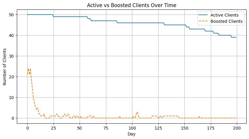
Fig. 18.6 Number of clients who at a given time are boosting their rates of requesting RfQs ten-fold vs the number of client actives. Clients become boosted when they receive prices from the dealer that are 35% cheaper than their reservation prices, and revert back to normal when they receive quotes worse than 50% of their reservation price. As in the previous section, they become inactive if their hit rate with the dealer is below 10% over the last 10 days.#
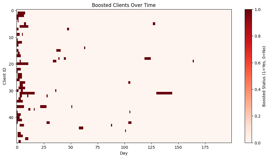
Fig. 18.7 Boosted clients over the simulation period. Each row represents a different client from the 50 ones simulated. Given the initial prior from the dealer regarding the reservation prices, which is too conservative, at the beginning of the simulation there is higher proportion of clients boosted, stabilizing after 25 days approximately.#
We estimate the model using the first 100 days of simulation, although we exclude the first 25 days to ensure the training data only uses a stable regime. The following plot shows the two estimated Beta density functions. Here, \(q_g = 89%\), which supports our hypothesis that the bad data density captures anomalies. This is also seen in the plot: on the one hand, the good data density captures the normal trading behavior concentrated around a region of probability of requesting RfQs, which actually becomes essentially Gaussian, given the high values of \(\alpha_g\) and \(\beta_g\); this is not the case for the bad data density, which takes a U-shape where most of the probability is concentrated around the extreme values. This reflects the two patterns of abnormal behavior present in our simulation, namely inactivity and boosted activity.
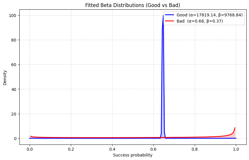
Fig. 18.8 Probability densities for the god and bad components of the model. The good data density is highly concentrated around a range of trading probabilities, becoming essentially a Gaussian distribution. The bad data density, on the other hand, places most of its density in the extreme values of very high and very low trading activity. The probability \(q_g\) equals 89% when fitted to the data, reflecting that bad data captures anomalies.#
With the model estimated, we use a 10 days window of days to compute the probability of abnormal client behavior over the second half of the dataset. This means that we only compute results for the last 90 days, since 10 days are needed to gather sufficient data. Bear in mind that this is not necessary in a Bayesian paradigm, since we could perfectly get estimations for any window, including zero data –defaulting to the prior probability of the hypotheses \(q_g\). We choose a 50% threshold on \(P({\rm good} |D)\) to trigger alerts. Over a dataset of 50 clients and 90 days tested, i.e. 4500 points, the model produced 3,811 true negatives (correctly identifying normal cases) and 545 true positives (correctly identifying abnormal cases). It made 75 false positives (normal cases incorrectly flagged as abnormal) and 69 false negatives (abnormal cases missed). Overall, this means the global abnormality rule (inactive OR boosted) shows high specificity (≈ 98% of normal cases correctly classified) and strong sensitivity (≈ 89% of abnormal cases detected), with a relatively small number of errors on both sides. Therefore, the approach seems reliable at detecting abnormal clients while only rarely misclassifying normal ones.
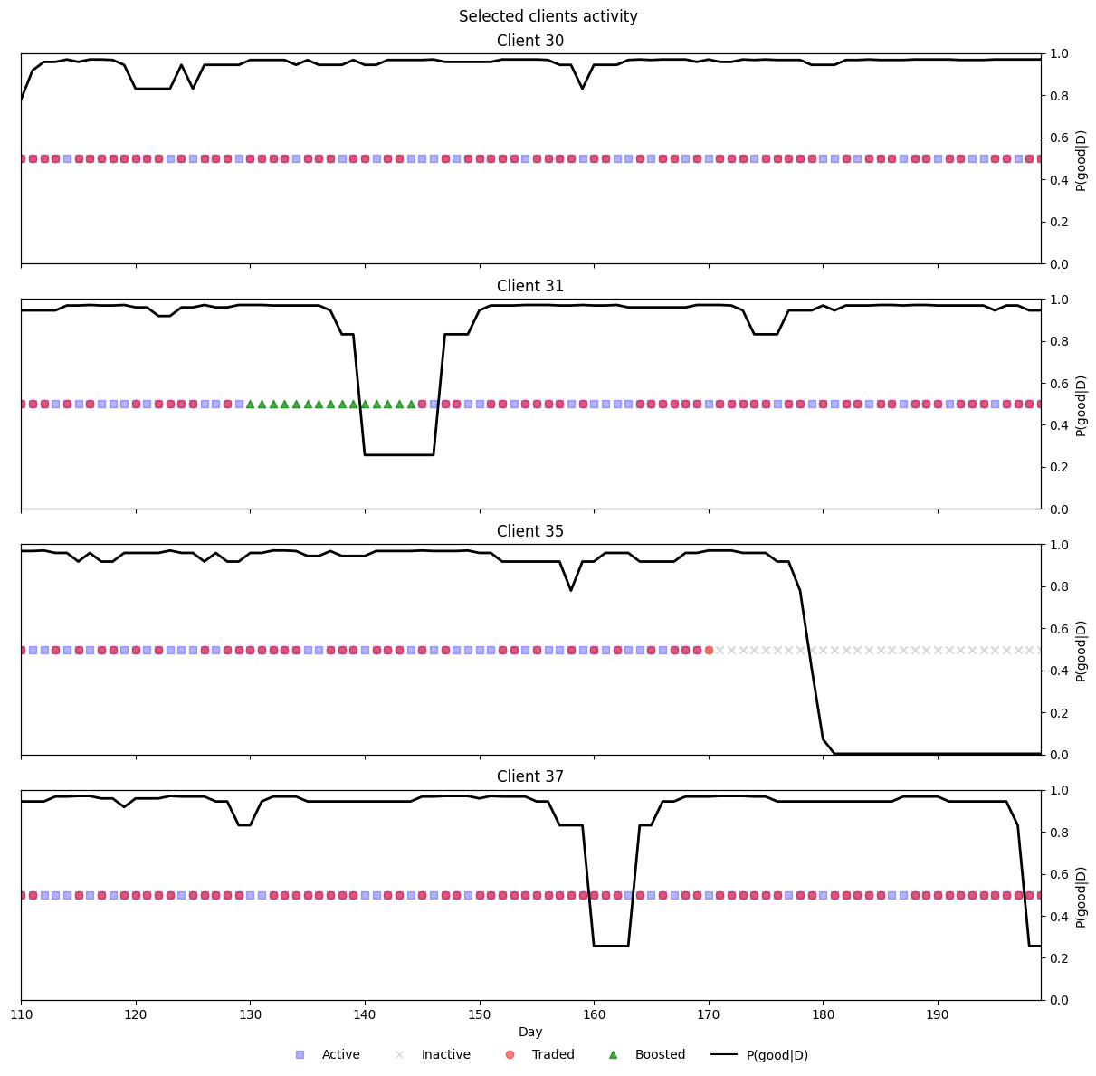
Fig. 18.9 Selected clients that showcase the different types of client behavior and how the model reacts to them.#
In the following figure we can see the predictions for specific clients showing different patterns of behavior:
Client 30: An example of a client with no abnormal trading behavior. The model correctly reflects this, keeping probabilities \(P({\rm good} |D)\) mostly above 80% and not triggering any alerts.
Client 31: Shows a period of boosted activity that the model captures after a few days, once sufficient evidence accumulates. When boosting ends, the probability quickly returns to high values after the first non-trading day, a pattern consistent with normality rather than extreme regimes. This illustrates the model’s asymmetry: it requires stronger evidence to reject normal trading (continuous activity can still occur under normal conditions) but reverts quickly once activity normalizes.
Client 35: Becomes inactive during the simulation. After eight consecutive days without trading, the model rejects the normal trading hypothesis and flags the client. As with Client 31, strong and sustained evidence (in this case, consecutive inactivity) is needed before the model issues an alert.
Client 37: Provides an instance of a false positive. A long, naturally occurring stretch of continuous activity was incorrectly flagged as abnormal. Since the model tends to produce confident abnormality probabilities quickly, one way to reduce such false positives—without significantly increasing false negatives—would be to lower the classification threshold.
In conclusion, despite its simplicity, the Good vs. Bad Data model performs well in identifying abnormal clients in the simulation, both those with unusually high trading activity and those with unusually low activity. For the latter, it performs on par with the attrition risk model presented earlier. Moreover, the framework could be extended into a multi-label classifier by comparing trading probabilities against the mean of the good-data cluster, issuing attrition risk alerts for unusually low activity and boosted activity alerts for the opposite case.
18.4. A Generative model for RfQs in negotiation#
18.5. Causal interventions#
18.5.1. Optimal pricing#
18.5.2. Axe matcher#
18.6. Exercises#
Prove the identity \(P(a = 1|D = 10100, p, \theta) = P(a = 1| D = 01100, p, \theta)\) by explicitly working out the second term in the equality.